\[ \begin{align}\begin{aligned}\newcommand{\bs}{\boldsymbol} \newcommand{\dp}{\displaystyle} \newcommand{\rm}{\mathrm} \newcommand{\cl}{\mathcal} \newcommand{\pd}{\partial}\\\newcommand{\cd}{\cdot} \newcommand{\cds}{\cdots} \newcommand{\dds}{\ddots} \newcommand{\lag}{\langle} \newcommand{\lv}{\lVert} \newcommand{\ol}{\overline} \newcommand{\od}{\odot} \newcommand{\ra}{\rightarrow} \newcommand{\rag}{\rangle} \newcommand{\rv}{\rVert} \newcommand{\seq}{\subseteq} \newcommand{\td}{\tilde} \newcommand{\vds}{\vdots} \newcommand{\wh}{\widehat}\\\newcommand{\0}{\boldsymbol{0}} \newcommand{\1}{\boldsymbol{1}} \newcommand{\a}{\boldsymbol{\mathrm{a}}} \newcommand{\b}{\boldsymbol{\mathrm{b}}} \newcommand{\c}{\boldsymbol{\mathrm{c}}} \newcommand{\d}{\boldsymbol{\mathrm{d}}} \newcommand{\e}{\boldsymbol{\mathrm{e}}} \newcommand{\f}{\boldsymbol{\mathrm{f}}} \newcommand{\g}{\boldsymbol{\mathrm{g}}} \newcommand{\h}{\boldsymbol{\mathrm{h}}} \newcommand{\i}{\boldsymbol{\mathrm{i}}} \newcommand{\j}{\boldsymbol{j}} \newcommand{\m}{\boldsymbol{\mathrm{m}}} \newcommand{\n}{\boldsymbol{\mathrm{n}}} \newcommand{\o}{\boldsymbol{\mathrm{o}}} \newcommand{\p}{\boldsymbol{\mathrm{p}}} \newcommand{\q}{\boldsymbol{\mathrm{q}}} \newcommand{\r}{\boldsymbol{\mathrm{r}}} \newcommand{\u}{\boldsymbol{\mathrm{u}}} \newcommand{\v}{\boldsymbol{\mathrm{v}}} \newcommand{\w}{\boldsymbol{\mathrm{w}}} \newcommand{\x}{\boldsymbol{\mathrm{x}}} \newcommand{\y}{\boldsymbol{\mathrm{y}}} \newcommand{\z}{\boldsymbol{\mathrm{z}}}\\\newcommand{\A}{\boldsymbol{\mathrm{A}}} \newcommand{\B}{\boldsymbol{\mathrm{B}}} \newcommand{\C}{\boldsymbol{\mathrm{C}}} \newcommand{\D}{\boldsymbol{\mathrm{D}}} \newcommand{\H}{\boldsymbol{\mathrm{H}}} \newcommand{\I}{\boldsymbol{\mathrm{I}}} \newcommand{\K}{\boldsymbol{\mathrm{K}}} \newcommand{\M}{\boldsymbol{\mathrm{M}}} \newcommand{\N}{\boldsymbol{\mathrm{N}}} \newcommand{\P}{\boldsymbol{\mathrm{P}}} \newcommand{\Q}{\boldsymbol{\mathrm{Q}}} \newcommand{\S}{\boldsymbol{\mathrm{S}}} \newcommand{\U}{\boldsymbol{\mathrm{U}}} \newcommand{\W}{\boldsymbol{\mathrm{W}}} \newcommand{\X}{\boldsymbol{\mathrm{X}}} \newcommand{\Y}{\boldsymbol{\mathrm{Y}}} \newcommand{\Z}{\boldsymbol{\mathrm{Z}}}\\\newcommand{\R}{\mathbb{R}}\\\newcommand{\cE}{\mathcal{E}} \newcommand{\cX}{\mathcal{X}} \newcommand{\cY}{\mathcal{Y}}\\\newcommand{\ld}{\lambda} \newcommand{\Ld}{\boldsymbol{\mathrm{\Lambda}}} \newcommand{\sg}{\sigma} \newcommand{\Sg}{\boldsymbol{\mathrm{\Sigma}}} \newcommand{\th}{\theta} \newcommand{\ve}{\varepsilon}\\\newcommand{\mmu}{\boldsymbol{\mu}} \newcommand{\ppi}{\boldsymbol{\pi}} \newcommand{\CC}{\mathcal{C}} \newcommand{\TT}{\mathcal{T}}\\ \newcommand{\bb}{\begin{bmatrix}} \newcommand{\eb}{\end{bmatrix}} \newcommand{\bp}{\begin{pmatrix}} \newcommand{\ep}{\end{pmatrix}} \newcommand{\bv}{\begin{vmatrix}} \newcommand{\ev}{\end{vmatrix}}\\\newcommand{\im}{^{-1}} \newcommand{\pr}{^{\prime}} \newcommand{\ppr}{^{\prime\prime}}\end{aligned}\end{align} \]

Chapter 18 Probabilistic Classification

18.1 Bayes Classifier

Let the training dataset \(\D\) consist of \(n\) points \(\x_i\) in a \(d\)-dimensional space, and let \(y_i\) denote the class for each point, with \(y_i\in\{c_1,c_2,\cds,c_k\}\). The Bayes classifier directly uses the Bayes theorem to predict the class for a new test instance, \(\x\). It estimates the posterior probability \(P(c_i|\x)\) for each class \(c_i\), and chooses the class that has the largest probability. The predicted class for \(\x\) is given as

\[\hat{y}=\arg\max_{c_i}\{P(c_i|\x)\}\]

The Bayes theorem allows us to invert the posterior probability in terms of the likelihood and prior probability, as follows:

Note

\(\dp P(c_i|\x)=\frac{P(\x|c_i)\cd P(c_i)}{P(\x)}\)

where \(P(\x|c_i)\) is the likelihood, defined as the probability of observing \(\x\) assuming that the true class is \(c_i\), \(P(c_i)\) is the prior probability of class \(c_i\), and \(P(\x)\) is the probability of observing \(\x\) from any of the \(k\) classes, given as

\[P(\x)=\sum_{j=1}^kP(\x|c_j)\cd P(c_j)\]

Because \(P(\x)\) is fixed for a given point, Bayes rule can be rewritten as

\[\hat{y}=\arg\max_{c_i}\{P(c_i|\x)\}=\arg\max_{c_i}\bigg\{\frac{P(\x|c_i)\cd P(c_i)}{P(\x)}\bigg\}\]

Note

\(\dp =\arg\max_{c_i}\{P(\x|c_i)P(c_i)\}\)

In other words, the predicted class essentially depends on the likelihood of that class taking its prior probability into account.

18.1.1 Estimating the Prior Probability

Let \(\D_i\) denote the subset of points in \(\D\) that are labeled with class \(c_i\):

\[\D_i=\{\x_j^T|\x_j\ rm{has\ class}\ y_i=c_i\}\]

Let the size of the dataset \(\D\) be given as \(|\D|=n\), and let the size of each class-specific subset \(\D_i\) be given as \(|D_i|=n_i\). The prior probability for class \(c_i\) can be estimated as follows:

Note

\(\dp\hat{P}(c_i)=\frac{n_i}{n}\)

18.1.2 Estimating the Likelihood

To estimate the likelihood \(P(\x|c_i)\), we have to estimate the joint probability of \(\x\) across all the \(d\) dimensions, that is, we have to estimate \(P(\x=(x_1,x_2,\cds,x_d)|c_i)\).

Numeric Attributes

In the parametric approach we typically assume that each class \(c_i\) is normally distributed around some mean \(\mmu_i\) with a corresponding covariance matrix \(\Sg_i\), both of which are estimated from \(\D_i\). For class \(c_i\), the probability density at \(\x\) is thus given as

Note

\(\dp f_i(\x)=f(\x|\mmu_i,\Sg_i)=\frac{1}{(\sqrt{2\pi})^d\sqrt{|\Sg_i|}}\) \(\dp\exp\bigg\{-\frac{(\x-\mmu_i)^T\Sg_i\im(\x-\mmu_i)}{2}\bigg\}\)

We can compute the likelihood by considiering a small interval \(\epsilon>0\) centered at \(\x\):

\[P(\x|c_i)=2\epsilon\cd f_i(\x)\]

The posterior probability is then given as

Note

\(\dp P(c_i|\x)=\frac{2\epsilon\cd f_i(\x)P(c_i)}{\Sg_{j=1}^k2\epsilon\cd f_j(\x)P(c_j)}\) \(\dp=\frac{f_i(\x)P(c_i)}{\Sg_{j=1}^kf_j(\x)P(c_j)}\)

Because \(\Sg_{j=1}^kf_j(\x)P(c_j)\) remain fixed for \(\x\), we can predict the class for \(\x\) by

\[\hat{y}=\arg\max_{c_i}\{f_i(\x)P(c_i)\}\]

The sample mean for the class \(c_i\) can be estimated as

\[\hat{\mmu_i}=\frac{1}{n_i}\Sg_{\x_j\in\D_i}\x_j\]

and the sample covariance matrix for each class can be estimated as

\[\hat{\Sg_i}=\frac{1}{n_i}\bar{\D_i}^T\bar{\D_i}\]

where \(\bar{\D_i}\) is the centered data matrix for class \(c_i\) given as \(\bar{\D_i}=\D_i-\1\cd\hat{\mmu_i}^T\). These values can be used to estimate the probability density as \(\hat{f_i}(\x)=f(\x|\hat{\mmu_i},\hat{\Sg_i})\).

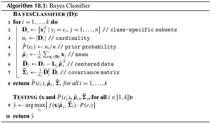
The cost of training is dominated by the covariance matrix computation step which takes \(O(nd^2)\) time.

Categorical Attributes

Let \(X_j\) be a categorical attribute over the domain \(dom(X_j)=\{a_{j1},a_{j2},\cds,a_{jm_j}\}\). Each categorical attributes \(X_j\) is modeled as an \(m_j\)-dimensional multivariate Bernoulli random variable \(\X_j\) that takes on \(m_j\) distinct vector values \(\e_{j1},\e_{j2},\cds,\e_{jm_j}\), where \(\e_{jr}\) is the \(r\)th standard basis vector in \(\R^{m_j}\) and corresponds to the \(r\)th value or symbol \(a_{jr}\in dom(X_j)\). The entire \(d\)-dimensional dataset is modeled as the vector random variable \(\X=(\X_1,\X_2,\cds,\X_d)^T\). Let \(d\pr=\sum_{j=1}^dm_j\); a categorical point \(\x=(x_1,x_2,\cds,x_d)^T\) is therefore represented as the \(d\pr\)-dimensional binary vector

\[\begin{split}\v=\bp \v_1\\\vds\\\v_d \ep=\bp \e_{1r_1}\\\vds\\\e_{dr_d} \ep\end{split}\]

where \(\v_j=\e_{jr_j}\) provided \(x_j=a_{jr_j}\) is the \(r_j\)th value in the domain of \(X_j\). The probability of the categorical point \(\x\) is obtained from the joint probability mass function (PMF) for the vector random variable \(\X\):

Note

\(P(\x|c_i)=f(\v|c_i)=f(\X_1=\e_1{r_1},\cds,\X_d=\e_{dr_d}|c_i)\)

The above joint PMF can be estimated directly from the data \(\D_i\) for each class \(c_i\) as follows:

\[\hat{f}(\v|c_i)=\frac{n_i(\v)}{n_i}\]

where \(n_i(\v)\) is the number of times the value \(\v\) occurs in class \(c_i\). Unfortuantely, if the probability mass at the point \(\v\) is zero for one or both classes, it would lead to a zero value for the posterior probability. One simple solution is to assume a pseudo-count 1 for each value, that is, to assume that each value of \(\X\) occurs at least one time, and to augment this base count of 1 with the actual number of occurrences of the observed value \(\v\) in class \(c_i\). The adjusted probability mass at \(\v\) is then given as

Note

\(\dp\hat{f}(\v|c_i)=\frac{n_i(\v)+1}{n_i+\prod_{j=1}^dm_j}\)

Challenges

The main problem with the Bayes classifier is the lack of enough data to reliably estimate the joint probability density or mass function, especially for high-dimensional data.

18.2 Naive Bayes Classifier

The naive Bayes approach makes the simple assumption that all the attributes are independent.

Note

\(\dp P(\x|c_i)=P(x_1,x_2,\cds,x_d|c_i)=\prod_{j=1}^dP(x_j|c_i)\)

Numeric Attributes

For numeric attributes we make the default assumption that each of them is normally distributed for each class \(c_i\). Let \(\mu_{ij}\) and \(\sg_{ij}^2\) denote the mean and variance for attribute \(X_j\), for class \(c_i\). The likelihood for class \(c_i\), for dimension \(X_j\), is given as

\[p(x_j|c_i)\varpropto f(x_j|\mu_{ij},\sg_{ij}^2)=\frac{1} {\sqrt{2\pi}\sg_{ij}}\exp\bigg\{-\frac{(x_j-\mu_{ij})^2}{2\sg_{ij}^2}\bigg\}\]

Incidentallly, the naive assumption corresponds to setting all the covariances to zero in \(\Sg_i\), that is,

\[\begin{split}\Sg_i=\bp\sg_{i1}^2&0&\cds&0\\0&\sg_{12}^2&\cds&0\\\vds&\vds&\dds&\vds\\0&0&\cds&\sg_{id}^2\ep\end{split}\]

This yields

\[|\Sg_i|=\det(\Sg_i)=\sg_{i1}^2\sg_{i2}^2\cds\sg_{id}^2=\prod_{j=1}^d\sg_{ij}^2\]

\[(\x-\mmu_i)^T\Sg_i\im(\x-\mmu_i)=\sum_{j=1}^d\frac{(x_j-\mu_{ij})^2}{\sg_{ij}^2}\]

\[ \begin{align}\begin{aligned}P(\x|c_i)&=\frac{1}{(\sqrt{2\pi})^d\sqrt{\prod_{j=1}^d\sg_{ij}^2}} \exp\bigg\{-\sum_{j=1}^d\frac{(x_j-\mu_{ij})^2}{2\sg_{ij}^2}\bigg\}\\&=\prod_{j=1}^d\bigg(\frac{1}{\sqrt{2\pi}\sg_{ij}}\exp\bigg\{-\frac{x_i-\mu_{ij})^2}{2\sg_{ij}^2}\bigg\}\bigg)\\&=\prod_{j=1}^dP(\x_j|c_i)\end{aligned}\end{align} \]

The naive Bayes classifier uses the sample mean \(\hat{\mmu_i}=(\hat{\mu_{i1}},\cds,\hat{\mu_{id}})^T\) and a diagonal sample covariance matrix \(\hat{\Sg_i}=diag(\sg_{i1}^2,\cds,\sg_{id}^2)\) for each class \(c_i\). Thus, in total \(2d\) parameters have to be estimated, corresponding to the sample mean and sample variance for each dimension \(X_j\).

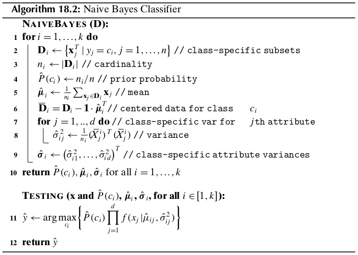
Training the naive Bayes classifier is very fast, with \(O(nd)\) computational complexity.

Categorical Attributes

Note

\(\dp P(\x|c_i)=\prod_{j=1}^dP(x_j|c_i)=\prod_{j=1}^df(\X_j=\e_{jr_j}|c_i)\)

where \(f(\X_j=\e_{jr_j}|c_i)\) is the probability mass function for \(\X_j\), which can be estimated from \(\D_i\) as follows:

\[\hat{f}(\v_j|c_i)=\frac{n_i(\v_j)}{n_i}\]

where \(n_i(\v_j)\) is the observed frequency of the value \(\v_j=\e_{jr_j}\) corresponding to the \(r_j\)th categorical value \(a_{jr_j}\) for the attribute \(X_j\) for class \(c_i\). The adjusted estimates with pseudo-counts are given as

Note

\(\dp\hat{f}(\v_j|c_i)=\frac{n_i(\v_j)+1}{n_i+m_j}\)

where \(m_j=|dom(X_j)|\).

18.3 \(K\) Nearest Neighbors Classifier

We illustrate the non-parameteric approach using nearest neighbors density estimation from Section 15.2.3, which leads to the K nearest neighbors (KNN) classifier.

Let \(\D\) be a training dataset comprising \(n\) points \(\x_i\in\R^d\), and let \(\D_i\) denote the subset of points in \(\D\) that are labeled with class \(c_i\), with \(n_i=|\D_i|\). Given a test point \(\x\in\R^d\), and \(K\), the number of neighbors to consider, let \(r\) denote the distance from \(\x\) to its \(K\)th nearest neighbor in \(\D\).

Consider the \(d\)-dimensional hyperball of radius \(r\) around the test point \(\x\), defined as

\[B_d(\x,r)=\{\x_i\in\D|\lv\x-\x_i\rv\leq r\}\]

We assume that \(|B_d(\x,r)|=K\).

Let \(K_i\) denote the number of points among the \(K\) nearest neighbors of \(\x\) that are labeled with class \(c_i\), that is

\[K_i=\{\x_j\in B_d(\x,r)|y_i=c_i\}\]

The class conditional probability density at \(\x\) can be estimated as the fraction of points from class \(c_i\) that lie within the hyperball divided by its volume, that is

Note

\(\dp\hat{f}(\x|c_i)=\frac{K_i/n_i}{V}=\frac{K_i}{n_iV}\)

where \(V=vol(B_d(\x,r))\) is the volume of the \(d\)-dimensional hyperball.

\[P(c_i|\x)=\frac{\hat{f}(\x|c_i)\hat{P}(c_i)}{\sum_{j=1}^k\hat{f}(\x|c_j)\hat{P}(c_j)}\]

\[\hat{f}(\x|c_i)\hat{P}(c_i)=\frac{K_i}{n_iV}\cd\frac{n_i}{n}=\frac{K_i}{nV}\]

\[P(c_i|\x)=\frac{\frac{K_i}{nV}}{\sum_{j=1}^k\frac{K_j}{nV}}=\frac{K_i}{K}\]

Note

\(\dp\hat{y}=\arg\max_{c_i}\{P(c_i|\x)\}=\arg\max_{c_i}\bigg\{\frac{K_i}{K}\bigg\}=\arg\max_{c_i}\{K_i\}\)

Beceause \(K\) is fixed, the KNN classifier predicts the class of \(\x\) as the majority class among its \(K\) nearest neighbors.