Chapter 4 Graph Data
4.1 Graph Concepts
Graph
A graph \(G=(V,E)\) is a mathematical structure consisting of a finite nonempty set \(V\) of vertices or nodes, and a set \(E\seq V\times V\) of edges consisting of unordered pairs of vertices. An edge from a node to itself, \((v_i,v_i)\), is called a loop. An undirected graph without loops is called a simple graph. An edge \(e=(v_i,v_j)\) between \(v_i\) and \(v_j\) is said to be incident with nodes \(v_i\) and \(v_j\) and \(v_j\) are adjacent to one another, and that they are neighbors. The number of nodes in the graph \(G\), given as \(|V|=n\) is called the order of the graph, and the number of edges in the graph, given as \(|E|=m\), is called the size of \(G\).
A directed graph or digraph has an edge set \(E\) consisting of ordered pairs of vertices. A directed edge \((v_i,v_j)\) is also called an arc, and is said to be from \(v_i\) to \(v_j\). We also say that \(v_i\) is the tail and \(v_j\) the head of the arc.
A weight graph consists of a graph together with a weight \(w_{ij}\) for each edge \((v_i,v_j)\in E\).
Subgraphs
A graph \(H=(V_H,E_H)\) is called a subgraph of \(G=(V,E)\) if \(V_H\seq V\) and \(E_H\seq E\). We also say that \(G\) is a supergraph of \(H\). Given a subset of the vertices \(V\pr\seq V\), the induced subgraph \(G\pr=(V\pr,E\pr)\) consists exactly of all the edges present in \(G\) between vertices in \(V\pr\). A (sub)graph is called complete (or a clique) if there exists an edge between all pairs of nodes.
Degree
The degree of a node \(v_i\in V\) is the number of edges incident with it, and is denoted as \(d(v_i)\) or just \(d_i\). The degree sequence of a graph is the list of the degrees of the nodes sorted in non-increasing order.
Let \(N_k\) denote the number of vertices with degree \(k\). The degree frequency distribution of a graph is given as
where \(t\) is the maximum degree for a node in \(G\). Let \(X\) be a random variable donoting the degree of a node. The degree distribution of a graph gives the probability mass function \(f\) for \(X\), given as
where \(f(k)=P(X=k)=\frac{N_k}{n}\) is the probability of a node with degree \(k\).
For directed graphs, the indegree of node \(v_i\) denoted as \(id(v_i)\), is the number of edges with \(v_i\) as head, that is, the number of incoming edges at \(v_i\). The outdegree of \(v_i\), denoted \(od(v_i)\), is the number of edges with \(v_i\) as the tail, that is, the number of outgoing edges from \(v_i\).
Path and Distance
A walk in a graph \(G\) between nodes \(x\) and \(y\) is an ordered sequence of vertices, starting at \(x\) and ending at \(y\),
such that there is an edge between every pair of consecutive verices, that is \((v_{i-1},v_i)\in E\) for all \(i=1,2,\cds,t\). The length of the walk, \(t\), is measured in terms of hops–the number of edges along the walk. Both the vertices and edges may be repeated in a walk. A walk starting and ending at the same vertex is called closed. A trail is a walk with distinct edges, and a path is a walk with distinct vertices (with the exception of the start and end vertices). A closed path with length \(t\geq 3\) is called a cycle.
A path of minumum length between nodes \(x\) and \(y\) is called a shortest path, and the length of the shortest path is called the distance between \(x\) and \(y\), denoted as \(d(x,y)\). If no path exists between the two nodes, the distance is assumed to be \(d(x,y)=\infty\).
Connectedness
Two nodes \(v_i\) and \(v_j\) are said to be connected if there exists a path between them. A graph is connected if there is a path between all pairs of vertices. A connected component, or just component, of a graph is a maximal connected subgraph. If a graph has only one component it is connected; otherwise it is disconnected.
For a directed graph, we say that it is strongly connected if there is a (directed) path between all ordered pairs of vertices. We say that it is weakly connected if there exists a path between node pairs only by considering edges as undirected.
Adjacency Matrix
A graph \(G=(V,E)\), with \(|V|=n\) vertices, can be conveniently represented in the form of an \(n\times n\), symmetric binary adjacency matrix, \(\A\), defined as
Note
\(\A(i,j)=\left\{\begin{array}{lr}1\quad\rm{if\ }v_i\rm{\ is\ adjacent\ to\ }v_j\\0\quad\rm{otherwise}\end{array}\right.\)
If the graph is directed, then the adjacency matrix \(\A\) is not symmetric, as \((v_i,v_j)\in E\) does not imply that \((v_j,v_i)\in E\).
If the graph is weighted, then we obtain an \(n\times n\) weighted adjacency matrix, \(\A\), defined as
Note
\(\A(i,j)=\left\{\begin{array}{lr}w_{ij}\quad\rm{if\ }v_i\rm{\ is\ adjacent\ to\ }v_j\\0\quad\rm{otherwise}\end{array}\right.\)
where \(w_{ij}\) is the weight on edge \((v_i,v_j)\in E\). A weighted adjacency matrix can always be converted into a binary one, if desired, by using some threshold \(\tau\) on the edge weights
Graph from Data Matrix
Let \(\D\) be a dataset consisting of \(n\) points \(\x_i\in\R^d\) in a \(d\)-dimensional space. We can define a weighted graph \(G=(V,E)\), where there exists a node for each point in \(\D\), and there exists a node for each point in \(\D\), and there exists an edge between each pair of points, with weight
where \(sim(\x_i,\x_j)\) denotes the similarity between points \(\x_i\) and \(\x_j\). For instance, similarity can be defined as being inversely related to the Euclidean distance between the points via the transformation
where \(\sg\) is the spread parameter.
4.2 Topological Attributes
The topological attributes of graphs are local if they apply to only a single node, or global if they refer to the entire graph.
Degree
The degree of a node \(\v_i\) is defined as the number of its neighbors.
Note
\(\dp d_i=\sum_j\A(i,j)\)
One of the simplest global attribute is the average degree:
Note
\(\dp \mu_d=\frac{\sum_id_i}{n}\)
Average Path Length
The average path length, also called the characteristic path length, of a connected graph is given as
Note
\(\dp\mu_L=\frac{\sum_i\sum_{j>i}d(v_i,v_j)}{\bp n\\2 \ep}=\frac{2}{n(n-1)}\sum_i\sum_{j>i}d(v_i,v_j)\)
For a directed graph, the average is over all ordered pairs of vertices:
Note
\(\dp\mu_L=\frac{1}{n(n-1)}\sum_i\sum_jd(v_i,v_j)\)
For a disconnected graph the average is taken over only the connected pairs of vertices.
Eccentricity
The eccentricity of a node \(v_i\) is the maximum distance from \(v_i\) to any other node in the graph:
Note
\(\dp e(v_i)=\max_j\{d(v_i,v_j)\}\)
If the graph is disconnected the eccentricity is computed only over pairs of vertices with finite distance, that is, only for verticese connected by a path.
Radius and Diameter
The radius of a connected graph, denoted \(r(G)\), is the minimum eccentricity of any node in the graph:
Note
\(r(G)=\min_i\{e(v_i)\}=\min_i\{\max_j\{d(v_i,v_j)\}\}\)
The diameter, denoted \(d(G)\), is the maximum eccentricity of any vertex in the graph:
Note
\(d(G)=\max_i\{e(v_i)\}=\max_{i,j}\{d(v_i,v_j)\}\)
For a disconnected graph, the diameter is the maximum eccentricity over all the connected components of the graph.
The diameter of a graph \(G\) is sensitive to outliers. A more robust notion is effective diameter, defined as the minimum number of hops for which a large fraction, typically \(90\%\), of all connected pairs of nodes can reach each other.
Clustering Coefficient
The clustering coefficient of a node \(v_i\) is a measure of the density of edges in the neighborhood of \(v_i\). Let \(G_i=(V_i,E_i)\) be the subgraph induced by the neighbors of vertex \(v_i\). Note that \(v_i\notin V_i\), as we assume that \(G\) is simple. Let \(|V_i|=n_i\) be the number of neighbors of \(v_i\) and \(|E_i|=m_i\) be the number of edges among the neighbors of \(v_i\). The clustering coefficient of \(v_i\) is defined as
Note
\(\dp C(v_i)=\frac{\rm{no.\ of\ edges\ in\ }G_i}{\rm{maximum\ number\ of\ edges\ in\ }G_i}=\) \(\dp\frac{m_i}{\bp n_i\\2 \ep}=\frac{2\cd m_i}{n_i(n_i-1)}\)
The clustering coefficient of a graph \(G\) is simply the average clustering coefficient over all the nodes, given as
Note
\(\dp C(G)=\frac{1}{n}\sum_iC(v_i)\)
Because \(C(v_i)\) is well defined only for nodes with degree \(d(v_i)\geq 2\), we can define \(C(v_i)=0\) for nodes with degree less than 2.
Define the subgraph composed of the edges \((v_i,v_j)\) and \((v_i,v_k)\) to be a connected triple centered at \(v_i\). A connected triple centered at \(v_i\) that includes \((v_j,v_k)\) is called a triangle. The clustering coefficient of node \(v_i\) can be expressed as
The transitivity of the graph is defined as
Efficiency
The efficiency for a pair of nodes \(v_i\) and \(v_j\) is defined as \(\frac{1}{d(v_i,v_j)}\). If \(v_i\) and \(v_j\) are not connected, then \(d(v_i,v_j)=\infty\) and the efficiency is \(1/\infty=0\). The efficiency of a graph \(G\) is the average efficiency over all pairs of nodes, whether connected or not, given as
The maximum efficiency value is 1, which holds for a complete graph.
The local efficiency for a node \(v_i\) is defined as the efficiency of the subgraph \(G_i\) induced by the neighbors of \(v_i\).
4.3 Centrality Analysis
The notion of centrality is used to rank the vertices of a graph in terms of how “central” or important they are. A centrality can be formally defined as a function \(c:V\ra\R\), that induces a total order on \(V\). We say that \(v_i\) is at least as central as \(v_j\) if \(c(v_i)\geq c(v_j)\).
4.3.1 Basic Centralities
Degree Centrality
The simplest notion of centrality is the degree \(d_i\) of a vertex \(v_i\)–the higher the degree, the more important or central the vertex.
Eccentricity Centrality
Eccentricity centrality is defined as follows:
Note
\(\dp c(v_i)\frac{1}{e(v_i)}=\frac{1}{\max_j\{d(v_i,v_j)\}}\)
A node \(v_i\) that has the least eccentricity, that is, for which the eccentricity equals the graph radius, \(e(v_i)=r(G)\), is called a center node, whereas a node that has the highest eccentricity, that is, for which eccentricity equals the graph diameter, \(e(v_i)=d(G)\), is called a periphery node.
Eccentricity centrality is related to the problem of facility location, that is, choosing the optimum location for a resource or facility.
Closeness Centrality
Closeness centrality uses the sum of all the distances to rank how central a node is
Note
\(\dp c(v_i)=\frac{1}{\sum_jd(v_i,v_j)}\)
A node \(v_i\) with the smallest total distance, \(\sum_jd(v_i,v_j)\) is called the median node.
Betweenness Centrality
The Betweenness centrality measures how many shortest paths between all pairs of vertices include \(v_i\). This gives an indication as to the central “monitoring” role played by \(v_i\) for various pairs of nodes. Let \(\eta_{jk}\) denote the number of shortest paths between vertices \(v_j\) and \(v_k\), and let \(\eta_{jk}(v_j)\) denote the number of such paths that include or contain \(v_i\). Then the fraction of paths through \(v_i\) is denoted as
If the two vertices \(v_i\) and \(v_k\) are not connected, we assume \(\gamma_{jk}(v_i)=0\).
The betweenness centrality for a node \(v_i\) is defined as
Note
\(\dp c(v_i)=\sum_{j\neq i}\sum_{k\neq i,k>j}\gamma_{jk}(v_i)=\) \(\dp\sum_{j\neq i}\sum_{k\neq i,k>j}\frac{\eta_{jk}(v_i)}{\eta_{jk}}\)
4.3.2 Web Centralities
Prestige
Let \(G=(V,E)\) be a directed graph, with \(|V|=n\). The adjacency matrix of \(G\) is an \(n\times n\) asymmetric matrix \(\A\) given as
Let \(p(u)\) be a positive real number, called the prestige or eigenvector centrality score for node \(u\).
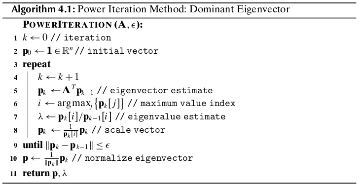
Across all the nodes, we can recursively express the prestige scores as
Note
\(\p\pr=\A^T\p\)
where \(\p\) is an \(n\)-dimensional column vector corresponding to the prestige scores for each vertex.
The dominant eigenvector of \(\A^T\) and the corresponding eigenvalue can be computed using the power iteration approach.
PageRank
The PageRank of a Web page is defined to be the probability of a random web surfer landing at that page.
Normalized Prestige
We assume for the moment that each node \(u\) has outdegree at least 1. Let \(od(u)=\sum_v\A(u,v)\) denote the outdegree of node \(u\). Because a randodm surfer can choose among any of its outgoing links, if there is a link from \(u\) to \(v\), then the probability of visiting \(v\) from \(u\) is \(\frac{1}{od(u)}\)
Staring from an initial probability or PageRank \(p_0(u)\) for each node, such that
we can compute an updated PageRank vector for \(v\) as follows:
where \(\N\) is the normalized adjacency matrix of the graph, given as
Across all nodes, we can express the PageRank vector as follows:
Random Jumps
In the random surfing approach, there is a small probability of jumping from one node to any of the other nodes in the graph, even if they do not have a link between them. For the random surfer matrix, the outdegree of each node is \(od(u)=n\), and the probability of jumping from \(u\) to any node \(v\) is simply \(\frac{1}{od(u)}=\frac{1}{n}\). The PageRank can then be computed analogously as
where \(\N_r\) is the normalized adjacency matrix of the fully connected Web graph, given as
Across all the nodes the random jump PageRank vector can be represented as
PageRank
The full PageRank is computed by assuming that with some small probability, \(\alpha\), a random Web surfer jumps from the current node \(u\) to any other random node \(v\), and with probability \(1-\alpha\) the user follows an existing link from \(u\) to \(v\).
Note
\(\p\pr=(1-\alpha)\N^T\p+\alpha\N_r^T\p=((1-\alpha)\N^T+\alpha\N_r^T)\p=\bs{\rm{M}}^T\p\)
When a node \(u\) does not have any outgoing edges, that is, when \(od(u)=0\), it acts like a sink for the normalized prestige score, and it can only jump to another random node. Thus, we need to make sure that if \(od(u)=0\) then for the row corresponding to \(u\) in \(\bs{\rm{M}}\), denoted as \(\bs{\rm{M}}_u\), we set \(\alpha=1\), that is
Hub and Authority Scores
The authority score of a page is analogous to PageRank or prestige, and it depends on how many “good” pages point to it. The hub score of a page is based on how many “good” pages it points to.
We denote by \(a(u)\) the authority score and by \(h(u)\) the hub score of node \(u\).
In matrix notation, we obtain
Note
\(\a\pr=\A^T\bs{\rm{h}}\quad\bs{\rm{h}}\pr=\A\a\)
In fact, we can write the above recursively as follows:
In other words, as \(k\ra\infty\), the authority score converges to the dominant eigenvector of \(\A^T\A\), whereas the hub score converges to the dominant eigenvector of \(\A\A^T\).
4.4 Graph Models
Small-world Property
A graph \(G\) exhibits small-world behavior if the average path length \(\mu_L\) scales logarithmically with the number of nodes in the graph, that is, if
Note
\(\mu_L\varpropto\log n\)
A graph is said to have ultra-small-world property if the average path length is much smaller than \(\log n\), that is, if \(\mu_L\ll\log n\).
Scale-free Property
In many real-world graphs, the probability that a node has degree \(k\) satisfies the condition
Note
\(f(k)\varpropto k^{-\gamma}\)
Rewrite above equality by introducing a proportionality constant \(\alpha\) that does not depend on \(k\), that is
Then we have
which is the equation of a straight line in the log-log plot of \(k\) versus \(f(k)\), with \(-\gamma\) giving the slope of the line.
A power-law relationship leads to a scale-free or scale invariant behavior because scaling the argument by some constant \(c\) does not change the proportionality.
Clustering Effect
Real-world graphs often also exhibit a clustering effect, that is, two nodes are more likely to be connected if they share a common neighbor. The clustering effect is captured by a high clustering coefficient for the graph \(G\). Let \(C(k)\) denote the average clustering coefficient for all nodes with degree \(k\); then the clustering effect also manifests itself as a power-law relationship between \(C(k)\) and \(k\):
Note
\(C(k)\varpropto k^{-\gamma}\)
In other words, a log-log plot of \(j\) versus \(C(k)\) exhibits a straight line behavior with negative slop \(-\gamma\).
4.4.1 Erdös–Rényi Random Graph Model
The Erdös–Rényi(ER) model generates a random graph such that any of the possible graph with a fixed number of nodes and edges has equal probability of being chosen.
Let \(M\) denote the maximum number of edges possible among the \(n\) nodes, that is,
The ER model specifies a collection of graphs \(\cl{G}(n,m)\) with \(n\) nodes and \(m\) edges, such that each graph \(G\in\cl{G}\) has equal probability of being selected:
where \(\bp M\\m \ep\) is the number of possible graphs with \(m\) edges corresponding to the way s of choosing the \(m\) edges out of a total of \(M\) possible edges.
Let \(V=\{v_1,v_2,\cds,v_n\}\) denote the set of \(n\) nodes. The ER method chooses a random graph \(G=(V,E)=\cl{G}\) via a generative process. At each step, it randomly selects two distinct vertices \(v_i,v_j\in V\), and adds an edge \((v_i,v_j)\) to \(E\), provided the edge is not already in the graph \(G\). The process is repeated until exactly \(m\) edges have been added to the graph.
Let \(X\) be a random variable denoting the degree of a node for \(G\in\cl{G}\). Let \(p\) denote the probability of an edge in \(G\), which can be computed as
Average Degree
For any given node in \(G\) its degree can be at most \(n-1\).
Note
\(f(k)=P(X=k)=\bp n-1\\k \ep p^k(1-p)^{n-1-k}\)
The average degree \(\mu_d\) is then given as the expected value of \(X\):
We can also compute the variance of the degrees among the nodes by computing the variance of \(X\):
Degree Distribution
As \(n\ra\infty\) and \(p\ra 0\), the expected value and variance of \(X\) can be written as
In other words, for large and sparse graphs the expectation and variance of \(X\) are the same:
and the binomial distribution can be approximated by a Poisson distribution with parameter \(\ld\), give as
Note
\(\dp f(k)=\frac{\ld^ke^{-\ld}}{k!}\)
where \(\ld=np\) represents both the expected value and variance of the distribution. Using Stirling’s approximation of the factorial \(k!\simeq k^ke^{-k}\sqrt{2\pi k}\) we obtain
In other words, we have
for \(\alpha=\ld e=npe\). The ER random graph model is not adequate to describe real-world scale-free graphs.
Clustering Coefficient
Let us cosinder a node \(v_i\) in \(G\) with degree \(k\). The clustering coefficient of \(v_i\) is given as
where \(k=n_i\) also denotes the number of nodes and \(m_i\) denotes the number of edges in the subgraph induced by neighbors of \(v_i\). However, because \(p\) is the probability of an edge, the expected number of edges \(m_i\) among the neighbors of \(v_i\) is simply
Thus, we obtain
Note
\(\dp C(G)=\frac{1}{n}\sum_iC(v_i)=p\)
For sparse graphs we have \(p\ra 0\), which in turn implies that \(C(G)=C(v_i)\ra 0\).
Diameter
The expected degree of a node is \(\mu_d=\ld\), and we can estimate the number of nodes at a distance of \(k\) hops away from a starting node \(v_i\) as \(\ld^k\). However, because there are a total of \(n\) distinct vertices in the graph, we have
where \(t\) denotes the maximum number of hops from \(v_i\). We have
Because the path length from a node to the farthest node is bounded by \(t\), it follows that the diameter of the graph is also bounded by that value, that is,
Note
\(d(G)\varpropto\log n\)
4.4.2 Watts-Strogatz Small-world Graph Model
The WS model starts with a regular graph of degree \(2k\), where each node is connected to its \(k\) neighbors on the right and \(k\) neighbors on the left.
Clustering Coefficient and Diameter of Regular Graph
Consider the subgraph \(G_v\) induced by the \(2k\) neighbors of a node \(v\). The clustering coefficient of \(v\) is given as
where \(m_v\) is the actual number of edges, and \(M_v\) is the maximum possible number of edges, among the neighbors of \(v\).
The degree of any node in \(G_v\) that is \(i\) backbone hops away from \(v\) is given as
Because each edge contributes to the degree of its two incident nodes, summing the degrees of all neighbors of \(v\) to obtain
On the other hand, the number of possible edges among the \(2k\) neighbors of \(v\) is given as
The clustering coefficient of a node \(v\) is given as
Note
\(C(v)=\frac{m_v}{M_v}=\frac{3k-3}{4k-2}\)
As \(k\) increases, the clustering coefficient approahces \(\frac{3}{4}\).
The diameter of a regular WS graph is given as
Note
\(d(G)=\left\{\begin{array}{lr}\lceil\frac{n}{2k}\rceil\quad\rm{if\ }n\rm{\ is\ even}\\\lceil\frac{n-1}{2k}\rceil\quad\rm{if\ }n\rm{\ is\ odd}\end{array}\right.\)
Random Perturbation of Regular Graph
Edge Rewiring
For each \((u,v)\) in the graph, with probability \(r\), replace \(v\) with another randomly chosen node avoiding loops and duplicate edges. Because the WS regular graph has \(m=kn\) total edges, after rewiring, \(rm\) of the edges are random, and \((1-r)m\) are regular.
Edge shortcuts
Add a few shortcut edges between random pairs of nodes, with \(r\) being the probability, per edge, of adding a shortcut edge. The total number of randum shortcut edges added to the network is \(mr=knr\). The total number of edges in the graph is \(m+mr=(1+r)m=(1+r)kn\).
Properties of Watts-Strogatz Graphs
Degree Distribution
Let \(X\) denote the random variable denoting the number of shortcuts for each node. Then the probability of a node with \(j\) shortcut edges is given as
with \(E[X]=n\pr p=2kr\) and \(p=\frac{2kr}{n-2k-1}=\frac{2kr}{n\pr}\) The expected degree of each node in the network is therefore
It is clear that the degree distribution of the WS graph does not adhere to a power law. Thus, such networks are not scale-free.
Clustering Coefficient
The clustering coefficient is
For small values of \(r\) the clustering coefficient remains high.
Diameter
Small values of shortcut edge probability \(r\) are enough to reduce the diameter from \(O(n)\) to \(O(\log n)\).
4.4.3 Barabási–Albert Scale-free Model
The Barabási–Albert(BA) model tries to capture the scale-free degree distributions of real-world graphs via a generative process that adds new nodes and edges at each time step. The edge growth is based on the concept of preferential attachment; that is, edges from the new vertex are more likely to link to nodes with higher degrees.
Let \(G_t\) denote the graph at time \(t\), and let \(n_t\) denote the number of nodes, and \(m_t\) the number of edges in \(G_t\).
Initialization
The BA model starts with \(G_0\), with each node connected to its left and right neighbors in a circular layout. Thus \(m_0=n_0\).
Growth and Preferential Attachment
The BA model derives a new graph \(G_{t+1}\) from \(G_t\) by adding exactly one new node \(u\) and adding \(q\leq n_0\) new edges from \(u\) to \(q\) distinct nodes \(v_j\in G_t\), where node \(v_j\) is chosen with probability \(\pi_t(v_j)\) proportional to its degree in \(G_t\), given as
Degree Distribution
The degree distribution for BA graphs is given as
For constant \(q\) and large \(k\), the degree distribution scales as
Note
\(f(k)\varpropto k^{-3}\)
The BA model yields a power-law degree distribution with \(\gamma=3\), especially for large degrees.
Clustering Coefficient and Diameter
The diameter of BA graphs scales as
The expected clustering coefficient of the BA graphs scales as