\[ \begin{align}\begin{aligned}\newcommand{\bs}{\boldsymbol} \newcommand{\dp}{\displaystyle} \newcommand{\rm}{\mathrm} \newcommand{\cl}{\mathcal} \newcommand{\pd}{\partial}\\\newcommand{\cd}{\cdot} \newcommand{\cds}{\cdots} \newcommand{\dds}{\ddots} \newcommand{\lag}{\langle} \newcommand{\lv}{\lVert} \newcommand{\ol}{\overline} \newcommand{\od}{\odot} \newcommand{\ra}{\rightarrow} \newcommand{\rag}{\rangle} \newcommand{\rv}{\rVert} \newcommand{\seq}{\subseteq} \newcommand{\td}{\tilde} \newcommand{\vds}{\vdots} \newcommand{\wh}{\widehat}\\\newcommand{\0}{\boldsymbol{0}} \newcommand{\1}{\boldsymbol{1}} \newcommand{\a}{\boldsymbol{\mathrm{a}}} \newcommand{\b}{\boldsymbol{\mathrm{b}}} \newcommand{\c}{\boldsymbol{\mathrm{c}}} \newcommand{\d}{\boldsymbol{\mathrm{d}}} \newcommand{\e}{\boldsymbol{\mathrm{e}}} \newcommand{\f}{\boldsymbol{\mathrm{f}}} \newcommand{\g}{\boldsymbol{\mathrm{g}}} \newcommand{\h}{\boldsymbol{\mathrm{h}}} \newcommand{\i}{\boldsymbol{\mathrm{i}}} \newcommand{\j}{\boldsymbol{j}} \newcommand{\m}{\boldsymbol{\mathrm{m}}} \newcommand{\n}{\boldsymbol{\mathrm{n}}} \newcommand{\o}{\boldsymbol{\mathrm{o}}} \newcommand{\p}{\boldsymbol{\mathrm{p}}} \newcommand{\q}{\boldsymbol{\mathrm{q}}} \newcommand{\r}{\boldsymbol{\mathrm{r}}} \newcommand{\u}{\boldsymbol{\mathrm{u}}} \newcommand{\v}{\boldsymbol{\mathrm{v}}} \newcommand{\w}{\boldsymbol{\mathrm{w}}} \newcommand{\x}{\boldsymbol{\mathrm{x}}} \newcommand{\y}{\boldsymbol{\mathrm{y}}} \newcommand{\z}{\boldsymbol{\mathrm{z}}}\\\newcommand{\A}{\boldsymbol{\mathrm{A}}} \newcommand{\B}{\boldsymbol{\mathrm{B}}} \newcommand{\C}{\boldsymbol{\mathrm{C}}} \newcommand{\D}{\boldsymbol{\mathrm{D}}} \newcommand{\H}{\boldsymbol{\mathrm{H}}} \newcommand{\I}{\boldsymbol{\mathrm{I}}} \newcommand{\K}{\boldsymbol{\mathrm{K}}} \newcommand{\M}{\boldsymbol{\mathrm{M}}} \newcommand{\N}{\boldsymbol{\mathrm{N}}} \newcommand{\P}{\boldsymbol{\mathrm{P}}} \newcommand{\Q}{\boldsymbol{\mathrm{Q}}} \newcommand{\S}{\boldsymbol{\mathrm{S}}} \newcommand{\U}{\boldsymbol{\mathrm{U}}} \newcommand{\W}{\boldsymbol{\mathrm{W}}} \newcommand{\X}{\boldsymbol{\mathrm{X}}} \newcommand{\Y}{\boldsymbol{\mathrm{Y}}} \newcommand{\Z}{\boldsymbol{\mathrm{Z}}}\\\newcommand{\R}{\mathbb{R}}\\\newcommand{\cE}{\mathcal{E}} \newcommand{\cX}{\mathcal{X}} \newcommand{\cY}{\mathcal{Y}}\\\newcommand{\ld}{\lambda} \newcommand{\Ld}{\boldsymbol{\mathrm{\Lambda}}} \newcommand{\sg}{\sigma} \newcommand{\Sg}{\boldsymbol{\mathrm{\Sigma}}} \newcommand{\th}{\theta} \newcommand{\ve}{\varepsilon}\\\newcommand{\mmu}{\boldsymbol{\mu}} \newcommand{\ppi}{\boldsymbol{\pi}} \newcommand{\CC}{\mathcal{C}} \newcommand{\TT}{\mathcal{T}}\\ \newcommand{\bb}{\begin{bmatrix}} \newcommand{\eb}{\end{bmatrix}} \newcommand{\bp}{\begin{pmatrix}} \newcommand{\ep}{\end{pmatrix}} \newcommand{\bv}{\begin{vmatrix}} \newcommand{\ev}{\end{vmatrix}}\\\newcommand{\im}{^{-1}} \newcommand{\pr}{^{\prime}} \newcommand{\ppr}{^{\prime\prime}}\end{aligned}\end{align} \]

Chapter 25 Neural Networks

Artificial neural networks or simply neural networks are inspired by biological neuronal networks. Artifical neural networks are comprised of abstract neurons that try to mimic real neurons at a very high level. They can be described via a weighte directed graph \(G=(V,E)\), with each node \(v_i\in V\) representing a neuron, and each directed edge \((v_i,v_j)\in E\) representing a synaptic to dendritic connection from \(v_i\) to \(v_j\). The weight of the edge \(w_{ij}\) denotes the synaptic strength. Nerual networks are characterized by the type of activation function used to generate an output, and the architecture of the network in terms of how the nodes are interconnected.

25.1 Artificial Neuron: Activation Functions

A neuro \(z_k\) has incoming edges from neurons \(x_1,\cds,x_d\). Let \(x_i\) denotes neuron \(i\), and also the value of that neuron. The net input at \(z_k\), denoted \(net_k\), is given as the weighted sum

Note

\(net_k=b_k+\sum_{i=1}^dw_{ik}\cd x_i=b_k+\w^T\x\)

where \(\w_k=(w_{1k},w_{2k},\cds,w_{dk})^T\in\R^d\) and \(\x=(x_1,x_2,\cds,x_d)^T\in\R^d\) is an input point. Notice that \(x_0\) is a special bias neuron whose value is always fixed at 1, and the weight from \(x_0\) to \(z_k\) is \(b_k\), which specifies the bias term for the neuron. Finally, the output value of \(z_k\) is given as some activation function, \(f(\cd)\), applied to the net input at \(z_k\)

\[z_k=f(net_k)\]

The value \(z_k\) is then passed along the outgoing edges from \(z_k\) to other neurons.

Linear/Identity Function:

\[f(net_k)=net_k\]

Step Function:

\[\begin{split}f(net_k)=\left\{\begin{array}{lr}1\quad\rm{if\ }net_k\leq 0\\0\quad\rm{if\ }net_k>0\end{array}\right.\end{split}\]

Rectified Linear Unit (ReLU):

\[\begin{split}f(net_k)=\left\{\begin{array}{lr}1\quad\rm{if\ }net_k\leq 0\\net_k\quad\rm{if\ }net_k>0\end{array}\right.\end{split}\]

An alternative expression for the ReLU activation is given as \(f(net_k)=\max\{0,net_k\}\).

Sigmoid:

\[f(net_k)=\frac{1}{1+\exp\{-net_k\}}\]

Hyperbolic Tangent (tanh):

\[f(net_k)=\frac{\exp\{net_k\}-\exp\{-net_k\}}{\exp\{net_k\}+\exp\{-net_k\}}= \frac{\exp\{2\cd net_k\}-1}{\exp\{2\cd net_k\}+1}\]

Softmax:

Softmax is mainly used at the output layer in a neural network, and unlike the other functions it depends not only on the net input at neuron \(k\), but it depends on the net signal at all other neurons in the output layer. Thus, given the net input vector, \(\bs{\rm{net}}=(net_1,net_2,\cds,net_p)^T\), for all the \(p\) output neurons, the output of the softmax function for the \(k\)th neuron is given as

\[f(net_k|\bs{\rm{net}})=\frac{\exp\{net_k\}}{\sum_{i=1}^p\exp\{net_i\}}\]

25.1.1 Derivatives for Activation Functions

Linear/Identity Function:

\[\frac{\pd f(net_j)}{\pd net_j}=1\]

Step Function:

The step function has a derivative of 0 everywhere except for the discontinuity at 0, where the derivative is \(\infty\).

Rectified Linear Unit (ReLU):

\[\begin{split}\frac{\pd f(net_k)}{\pd net_j}=\left\{\begin{array}{lr}0\quad\rm{if\ }net_j\leq 0\\1\quad\rm{if\ }net_k>0\end{array}\right.\end{split}\]

At 0, we can set the derivative to be any value in the range \([0,1]\).

Sigmoid:

\[\frac{\pd f(net_j)}{\pd net_j}=f(net_j)\cd (1-f(net_j))\]

Hyperbolic Tangent (tanh):

\[\frac{\pd f(net_j)}{\pd net_j}=1-f(net_j)^2\]

Softmax:

Since softmax is used at the output layer, if we denote the \(i\)th output neuron as \(o_i\), then \(f(net_i)=o_i\).

\[\begin{split}\frac{\pd f(net_j|\bs{\rm{net}})}{\pd net_k}=\frac{\pd o_j}{\pd net_k}= \left\{\begin{array}{lr}o+j\cd(1-o_j)\quad\rm{if\ }k=j\\ -o_k\cd o_j\quad\quad\quad\quad\rm{if\ }k\ne j\end{array}\right.\end{split}\]

25.2 Neural Networks: Regression and Classification

25.2.1 Regression

Consider the multiple (linear) regression problem, where given an input \(\x_i\in\R^d\), the goal is to predict the response as follows:

\[\hat{y_i}=b+w_1x_{i1}+w_2x_{i2}+\cds+w_dx_{id}\]

Given a training data \(\D\) comprising \(n\) points \(\x_i\) in a \(d\)-dimensional space, along with their corresponding true response value \(y_i\), the bias and weights for linear regression are chosen so as to minimize the sum of squared errors between the true and predicted response over all data points

\[SSE=\sum_{i=1}^n(y_i-\hat{y_i})^2\]

A neural network with \(d+1\) input neurons \(x_0,x_1,\cds,x_d\), including the bias neuron \(x_0=1\), and a single output neuron \(o\), all with identity activation functions and with \(\hat{y}=o\), represents the exact same model as multiple linear regression. Wereas the multiple regression problem has a closed form solution, neural networks learn the bias and weights via a gradient descent approach that minimizes the squared error.

Neural networks can just as easily model the multivariate (linear) regression task, where we have a \(p\)-dimensional response vector \(\y_i\in\R^p\) instead of a single value \(y_i\). That is, the training data \(\D\) comprises \(n\) points \(\x_i\in\R^d\) and their true response vectors \(\y_i\in\R^p\). Multivariate regression can be modeled by a neural network with \(d+1\) input neurons, and \(p\) output neurons \(o_1,o_2,\cds,o_p\), with all input and output neurons using the identity activation function. A neural network learns the weights by comparing its predicted output \(\hat\y=\o=(o_1,o_2,\cds,o_p)^T\) with the true response vector \(\y=(y_1,y_2,\cds,y_p)^T\). That is, training happens by first computing the error function or loss function between \(\o\) and \(\y\). When the prediction matches the true output the loss should be zero. The most common loss function for regression is the squared error function

\[\cl{E}_\x=\frac{1}{2}\lv\y-\o\rv^2=\frac{1}{2}\sum_{j=1}^p(y_j-o_j)^2\]

where \(\cl{E}_\x\) denotes the error on input \(\x\). Across all the points in a dataset, the total sum of squared error is

\[\cl{E}=\sum_{i=1}^n\cl{E}_{\x_i}=\frac{1}{2}\cd\sum_{i=1}^n\lv\y_i-\o_i\rv^2\]

25.2.2 Classification

Consider the binary classification problem, where \(y=1\) dentoes that the point belongs to the positive class, and \(y=0\) means that it belongs to the negative class. In logistic regression, we model the probability of the positive class viar the logistic (or sigmoid) function:

\[ \begin{align}\begin{aligned}\pi(\x)=P(y=1|\x)=\frac{1}{1+\exp\{-(b+\w^T\x)\}}\\P(y=0|\x)=1-P(y=1|\x)=1-\pi(\x)\end{aligned}\end{align} \]

Given input \(\x\), true response \(y\), and predicted response \(o\), recall that the cross-entropy error is defined as

\[\cl{E}_\x=-(y\cd\ln(o)+(1-y)\cd\ln(1-o))\]

With sigmoid activation, the output of the neural network is given as

\[o=f(net_o)=\rm{sigmoid}(b+\w^T\x)=\frac{1}{1+\exp\{-(b+\w^T\x)\}=\pi(\x)\]

which is the same as the logstic regression model.

Multiclass Logistic Regression

For the general classification problem with \(K\) classes \(\{c_1,c_2,\cds,c_K\}\), the true response \(y\) is encoded as a one-hot vector. Thus, class \(c_i\) is encoded as \(\e_1=(1,0,\cds,0)^T\), and so on, with \(\e_1\in\{0,1\}^K\) for \(i=1,2,\cds,K\). Thus, we encode \(y\) as a multivariate vector \(\y\in\{\e_1,\e_2,\cds,\e_K\}\). Recall that in multiclass logistic regression the task is to estimate the per class bias \(b_i\) and weight vector \(\w_i\in\R^d\), with the last class \(c_K\) used as the base class with fixed bias \(b_K=0\) and fixed weight vector \(\w_K=(0,0,\cds,0)^T\in\R^d\). The probability vector across all \(K\) classes is modeled via the softmax function:

\[\pi_i(\x)=\frac{\exp\{b_i+\w_i^T\x\}}{\sum_{j=1}^K\exp\{b_J+\w_J^T\x\}},\ \rm{for\ all\ }i=1,2,\cds,K\]

Therefore, the neural network can solve the multiclass logistic regression task, provided we use a softmax activation at the outputs, and use the \(K\)-way cross-entropy error, defined as

\[\cl{E}_\x=-(y_1\cd\ln(o_1)+\cds+y_K\cd\ln(o_K))\]

where \(\x\) is an input vector, \(\o=(o_1,o_2,\cds,o_K)^T\) is the predicted response vector, and \(\y=(y_1,y_2,\cds,y_k)^T\) is the true response vector. Note that only one element of \(\y\) is 1, and the rest are 0, due to the one-hot encoding.

With softmax activation, the output of the neural network is given as

\[o_i=P(\y=\e_i|\x)=f(net_i|\bs{\rm{net}})=\frac{\exp\{net_i\}}{\sum_{j=1}^p\exp\{net_j\}}=\pi_i(\x)\]

The only restriction we have to impose on the neural network is that weights on edges into the last output neuron should be zero to model the base class weights \(\w_K\). However, in practice, we relax this restriction, and just learn a regular weight vector for class \(c_K\).

25.2.3 Error Functions

Squared Error:

Given an input vector \(\x\in\R^d\), the squared error loss function measures the squared deviation between the predicted output vector \(\o\in\R^p\) and the true response \(\y\in\R^p\), defined as follows:

Note

\(\dp\cl{E}_\x=\frac{1}{2}\lv\y-\o\rv^2=\frac{1}{2}\sum_{j=1}^p(y_j-o_j)^2\)

where \(\cl{E}_\x\) denotes the error on input \(\x\).

\[ \begin{align}\begin{aligned}\frac{\pd\cl{E}_\x}{\pd o_j}=\frac{1}{2}\cd 2\cd(y_j-o_j)\cd -1=o_j-y_j\\\frac{\pd\cl{E}_\x}{\pd\o}=\o-\y\end{aligned}\end{align} \]

Cross-Entropy Error:

For classification tasks, with \(K\) classes \(\{c_1,c_2,\cds,c_K\}\), we usually set the number of output neurons \(p=K\), with one output neuron per class. Furthermore, each of the classes is coded as a one-hot vector, with class \(c_i\) encoded as the \(i\)th standard basis vector \(\e_i=(e_{i1},e_{i2},\cds,e_{iK})^T\in\{0,1\}^K\), with \(e_{ii}=1\) and \(e_{ij}=0\) for all \(j\ne i\). Thus, given input \(\x\in\R^d\), with the true response \(\y=(y_1,y_2,\cds,y_K)^T\), where \(\y\in\{\e_1,\e_2,\cds,\e_K\}\), the cross-entropy loss is defined as

Note

\(\dp\cl{E}_\x=-\sum_{i=1}^Ky_i\cd\ln(o_i)=-(y_1\cd\ln(o_1)+\cds+y_K\cd\ln(o_K))\)

\[ \begin{align}\begin{aligned}\frac{\pd\cl{E}_\x}{\dp o_j}=-\frac{y_j}{o_j}\\\frac{\pd\cl{E}_\x}{\pd\o}=\bigg(\frac{\pd\cl{E}_\x}{\dp o_1}, \frac{\pd\cl{E}_\x}{\dp o_2},\cds,\frac{\pd\cl{E}_\x}{\dp o_K}\bigg)^T= \bigg(-\frac{y_1}{o_1},-\frac{y_2}{o_2},\cds,-\frac{y_K}{o_K}\bigg)^T\end{aligned}\end{align} \]

Binary Cross-Entropy Error:

For classification tasks with binary classes, it is typical to encode the positive class as 1 and the negative class as 0, as opposed to using a one-hot encoding as in the general \(K\)-class case. Given an input \(\x\in\R^d\), with true response \(y\in\{0,1\}\), there is only one output neuron \(o\). Therefore, the binary cross-entropy error is defined as

Note

\(\cl{E}_\x=-(y\cd\ln(o)+(1-y)\cd\ln(1-o))\)

\[ \begin{align}\begin{aligned}\frac{\pd}{\cl{E}_\x}&=\frac{\pd}{\pd o}\{y\cd\ln(o)-(1-y)\cd\ln(1-o)\}\\&=-\bigg(\frac{y}{o}+\frac{1-y}{1-o}\cd-1\bigg)=\frac{-y\cd(1-o)+(1-y)\cd o}{o\cd(1-o)}\\&=\frac{o-y}{o\cd(1-o)}\end{aligned}\end{align} \]

25.3 Multilayer Perceptron: One Hidden Layer

A multilayer perceptron (MLP) is a neural network that has distinct layers of neurons. The inputs to the neural network comprise the input layer, and the final outputs from the MLP comprise the output layer. Any intermediate layer is called a hidden layer, and an MLP can have one or many hidden layers. Networks with many hidden layers are called deep neural networks. An MLP is also a feed-forward network. Typically, MLPs are fully connected between layers.

25.3.1 Feed-forward Phase

Let \(\D\) denote the training dataset, comprising \(n\) input points \(\x_i\in\R^d\) and corresponding true response vectors \(\y_i\in\R^p\). For each pair \((\x,\y)\) in the data, in the feed-forward phase, the point \(\x=(x_1,x_2,\cds,x_d)^T\in\R^d\) is supplied as an input to the MLP.

Given the input neuron values, we compute the output value for each hidden neuron \(z_k\) as follows:

\[z_k=f(net_k)=f\bigg(b_K+\sum_{i=1}^dw_{ik}\cd x_i\bigg)\]

where \(w_{ik}\) denotes the weight between input neuron \(x_i\) and hidden neuron \(z_k\).

\[o_j=f(net_j)=f\bigg(b_j+\sum_{i=1}^mw_{ij}\cd z_i)\]

where \(w_{ij}\) denotes the weight between hidden neuron \(z_i\) and output neuron \(o_j\).

We define the \(d\times m\) matrix \(\W_h\) comprising the weights between input and hidden layer neurons, and vector \(\b_j\in\R^m\) comprising the bias terms for hidden layer neurons, given as

\[\begin{split}\W_h=\bp w_{11}&w_{12}&\cds&w_{1m}\\w_{21}&w_{22}&\cds&w_{2m}\\\vds&\vds& \dds&\vds\\w_{d1}&w_{d2}&\cds&w_{dm}\ep\quad\b_h=\bp b_1\\b_2\\\vds\\b_m\ep\end{split}\]

where \(w_{ij}\) denotes the weight on the edge between input neuron \(x_i\) and hidden neuron \(z_j\), and \(b_i\) denotes the bias weight from \(x_0\) to \(z_i\).

Note

\(\bs{\rm{net}}_h=\b_h+\W_h^T\x\)

\(\z=f(\bs{\rm{net}}_h=f(\b_h+\w_h^T\x)\)

Here, \(\bs{\rm{net}}_h=(net_1,\cds,net_m)^T\) denotes the net input at each hidden neuron, and \(\z=(z_1,z_2,\cds,z_m)^T\) denotes the vector of hidden neuron values.

Likewise, let \(\W_o\in\R^{m\times p}\) denote the weight matrix between the hidden and output layers, and let \(\b_o\in\R^p\) be the bias vector for output neurons, given as

\[\begin{split}\W_o=\bp w_{11}&w_{12}&\cds&w_{1p}\\w_{21}&w_{22}&\cds&w_{2p}\\\vds&\vds& \dds&\vds\\w_{m1}&w_{m2}&\cds&w_{mp}\ep\quad\b_h=\bp b_1\\b_2\\\vds\\b_p\ep\end{split}\]

Note

\(\bs{\rm{net}}_o=\b_o+\W_o^T\z\)

\(\o=f(\bs{\rm{net}}_o=f(\b_o+\w_o^T\z)\)

\[\o=f(\b_o+\w_o^T\z)=f(\b_o+\W_o^T\cd f(\b_h+\W_h^T\x))\]

25.3.2 Backpropagation Phase

For a given input pair \((\x,\y)\) in the training data, the MLP first computes the output vector \(\o\) via the feed-forward step. Next, it computes the error in the predicted output vis-a-vis the true response \(\y\) using the squared error function

\[\cl{E}_\x=\frac{1}{2}\lv\y-\o\rv^2=\frac{1}{2}\sum_{j=1}^p(y_j-o_j)^2\]

The weight update is done via a gradient descent approach to minimize the error. Let \(\nabla_{w_{ij}}\) be the gradient of the error function with respect to \(w_{ij}\), or simply the weight gradient at \(w_{ij}\). Given the previous weight estimate \(w_{ij}\), a new weight is computed by taking a small step \(\eta\) in a direction that is opposite to the weight gradient at \(w_{ij}\)

\[w_{ij}=w_{ij}-\eta\cd\nabla_{w_{ij}}\]

In a similar manner, the bias term \(b_j\) is also updated via gradient descent

\[b_j=b_j-\eta\cd\nabla_{b_j}\]

where \(\nabla_{b_j}\) is the gradient of the error function with respect to \(b_j\), which we call the bias gradient at \(b_j\).

Updating Parameters Between Hidden and Output Layer

\[ \begin{align}\begin{aligned}\nabla_{w_{ij}}&=\frac{\pd\cl{E}_\x}{\pd w_{ij}}=\frac{\pd\cl{E}_\x} {\pd net_j}\cd\frac{\pd net_j}{\pd w_{ij}}=\delta_j\cd z_i\\\nabla_{b_j}&=\frac{\pd\cl{E}_\x}{\pd b_j}=\frac{\pd\cl{E}_\x}{\pd net_j}\cd \frac{\pd net_j}{\pd b_j}=\delta_j\end{aligned}\end{align} \]

where we use the symbol \(\delta_j\) to denote the partial derivative of the error with respect to net signal at \(o_j\), which we also call the net gradient at \(o_j\)

\[\delta_j=\frac{\pd\cl{E}_\x}{\pd net_j}\]

Futhermore, the partial derivative of \(net_j\) with respect to \(w_{ij}\) and \(b_j\) is given as

\[\frac{\pd net_j}{\pd w_{ij}}=\frac{\pd}{\pd w_{ij}}\bigg\{b_j+\sum_{k=1}^m w_{kj}\cd z_k\bigg\}=z_i\quad\quad\frac{\pd net_j}{\pd b_j}=\frac{\pd} {\pd b_j}\bigg\{b_j+\sum_{k=1}^mw_{kj}\cd z_k\bigg\}=1\]

\[\delta_j=\frac{\pd\cl{E}_\x}{\pd net_j}=\frac{\pd\cl{E}_\x}{\pd f(net_j)}\cd\frac{\pd f(net_j)}{\pd net_j}\]

Note that \(f(net_j)=o_j\), we have

\[\frac{\pd\cl{E}_\x}{\pd f(net_j)}=\frac{\pd\cl{E}_\x}{\pd o_j}=\frac{\pd} {\pd o_j}\bigg\{\frac{1}{2}\sum_{k=1}^p(y_k-o_k)^2\bigg\}=(o_j-y_j)\]

\[\frac{\pd f(net_j)}{\pd net_j}=o_j\cd(1-o_j)\]

Putting it all together, we get

\[\delta_j=(o_j-y_j)\cd o_j\cd(1-o_j)\]

Let \(\bs\delta_o=(\delta_1,\delta_2,\cds,\delta_p)^T\) denote the vector of net gradients at each output neuron, which we call the net gradient vector for the output layer. We can write \(\bs\delta_o\) as

Note

\(\bs\delta_o=\o\od(\1-\o)\od(\o-\y)\)

where \(\od\) denotes the element-wise product (also called the Hadamard product) between the vectors.

Let \(\z=(z_1,z_2,\cds,z_m)^T\) denote the vector comprising the values of all hidden layer neurons (after applying the activation function). We can compute the gradients \(\delta_{w_{ij}}\) for all hidden to output neuron connections via the outer product of \(\z\) and \(\bs\delta_o\):

Note

\(\dp\bs\nabla_{\W_o}=\bp\delta_{w_{11}}&\delta_{w_{12}}&\cds&\delta_{w_{1p}}\\\delta_{w_{21}}&\delta_{w_{22}}&\cds&\delta_{w_{2p}}\\\vds&\vds&\dds&\vds\\\delta_{w_{m1}}&\delta_{w_{m2}}&\cds&\delta_{w_{mp}}\ep=\z\cd\bs\delta_o^T\)

The vector of bias gradients is given as:

Note

\(\bs\nabla_{\b_o}=(\nabla_{b_1},\nabla_{b_2},\cds,\nabla_{b_p})^T=\bs\delta_o\)

Note

\(\W_o=\W_o-\eta\cd\bs\nabla_{\w_o}\)

\(\b_o=\b_o-\eta\cd\nabla_{\b_o}\)

Updating Parameters Between Input and Hidden Layer

\[ \begin{align}\begin{aligned}\nabla_{w_{ij}}&=\frac{\pd\cl{E}_\x}{\pd w_{ij}}=\frac{\pd\cl{E}_\x} {\pd net_j}\cd\frac{\pd net_j}{\pd w_{ij}}=\delta_j\cd x_i\\\nabla_{b_j}&=\frac{\pd\cl{E}_\x}{\pd b_j}=\frac{\pd\cl{E}_\x}{\pd net_j}\cd \frac{\pd net_j}{\pd b_j}=\delta_j\end{aligned}\end{align} \]

which follows from

\[\frac{\pd net_j}{\pd w_{ij}}=\frac{\pd}{\pd w_{ij}}\bigg\{b_j+\sum_{k=1}^m w_{kj}\cd x_k\bigg\}=x_i\quad\quad\frac{\pd net_j}{\pd b_j}=\frac{\pd} {\pd b_j}\bigg\{b_j+\sum_{k=1}^mw_{kj}\cd x_k\bigg\}=1\]

\[ \begin{align}\begin{aligned}\delta_j&=\frac{\pd\cl{E}_\x}{\pd net_j}=\sum_{k=1}^p\frac{\pd\cl{E}_\x} {\pd net_k}\cd\frac{\pd net_k}{\pd z_j}\cd\frac{\pd z_j}{\pd net_j}= \frac{\pd z_j}{\pd net_j}\cd\sum_{k=1}^p\frac{\pd\cl{E}_\x}{\pd net_k}\cd \frac{\pd net_k}{\pd z_j}\\&=z_j\cd(1-z_j)\cd\sum_{k=1}^p\delta_k\cd w_{jk}\end{aligned}\end{align} \]

where \(\frac{\pd z_j}{\pd net_j}=z_j\cd(1-z_j)\), since we assume a sigmoid activation function for the hidden neurons.

Let \(\bs\delta_o=(\delta_1,\delta_2,\cds,\delta_p)^T\) denote the vector of net gradients at the output nerurons, and \(\bs\delta_h=(\delta_1,\delta_2,\cds,\delta_m)^T\) the net gradients at the hidden layer neurons. We can write \(\bs\delta_h\) compactly as

Note

\(\bs\delta_h=\z\od(\1-\z)\od(\W_o\cd\bs\delta_o)\)

Furthermore, \(\W_o\cd\bs\delta_o\in\R^m\) is the vector of weighted gradients at each hidden neuron, since

\[\W_o\cd\bs\delta_o=\bigg(\sum_{k=1}^p\delta_k\cd w_{1k},\sum_{k=1}^p\delta_k \cd w_{2k},\cds,\sum_{k=1}^p\delta_k\cd w_{mk}\bigg)^T\]

Let \(\x=(x_1,x_2,\cds,x_d)^T\) denote the input vector, we can compute the gradients \(\nabla_{w_{ij}}\) for all input to hidden layer connections via the outer product:

Note

\(\dp\bs\nabla_{\W_h}=\bp\delta_{w_{11}}&\delta_{w_{12}}&\cds&\delta_{w_{1m}}\\\delta_{w_{21}}&\delta_{w_{22}}&\cds&\delta_{w_{2m}}\\\vds&\vds&\dds&\vds\\\delta_{w_{d1}}&\delta_{w_{d2}}&\cds&\delta_{w_{dm}}\ep=\x\cd\bs\delta_h^T\)

The vector of bias gradients is given as:

Note

\(\nabla_{\b_j}=(\nabla_{b1},\nabla_{b2},\cds,\nabla_{bm})^T=\bs\delta_h\)

Note

\(\W_h=\W_h-\eta\cd\bs\nabla_{\W_h}\)

\(\b_h=\b_h-\eta\cd\nabla_{\b_h}\)

25.3.3 MLP Training

The total training time per iteration is \(O(dm+mp)\).

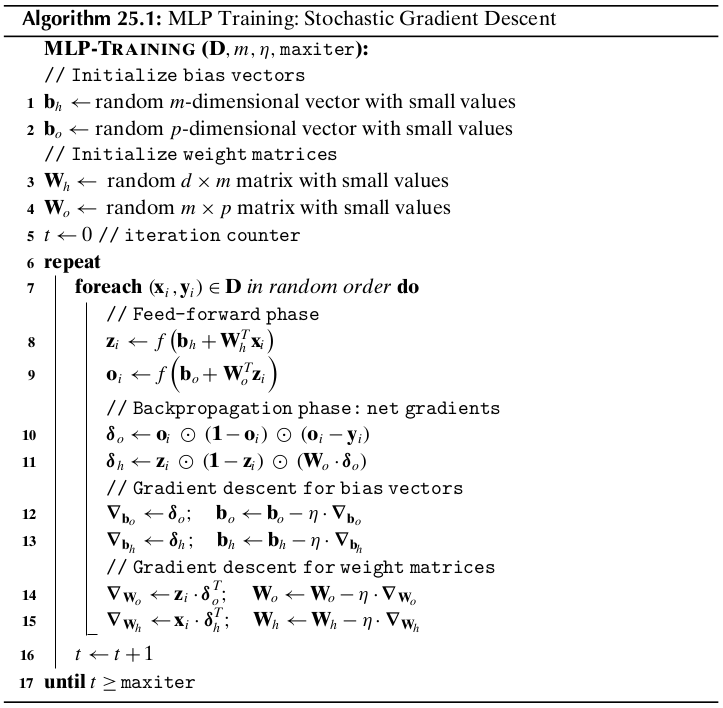
25.4 Deep Multilayer Perceptrons

Consider an MLP with \(h\) hidden layers. We assume that the input to the MLP comprises \(n\) points \(\x_i\in\R^d\) with the corresponding true response vector \(\y_i\in\R^p\). We denote the input neurons as layer \(l=0\), the first hidden layer as \(l=1\), the last hidden layer as \(l=h\), and the output layer as layer \(l=h+1\). We use \(n_l\) to denote the number of neurons in layer \(l\). We have \(n_0=d\), and \(n_{h+1}=p\). The vector of neuron values for layer \(l\) (for \(l=0,\cds,h+1\)) is denoted as

\[\z^l=(z_1^l,\cds,z_{n_l}^l)^T\]

Each layer except the output layer has one extra bias neuron, which is the neuron at index 0. Thus, the bias neuron for layer \(l\) is denoted \(z_0^l\) and its value is fixed at \(z_0^l=1\).

The vector of input neuron values is also written as

\[\x=(x_1,x_2,\cds,x_d)^T=(z_1^0,z_2^0,\cds,z_d^0)^T=\z^0\]

and the vector of output neuron values is also denoted as

\[\o=(o_1,o_2,\cds,o_p)^T=(z_1^{h+1},z_2^{h+1},\cds,z_p^{h+1})^T=\z^{h+1}\]

The weight matrix between layer \(l\) and layer \(l+1\) neurons is denoted \(\W_l\in\R^{n_l\times n_{l+1}}\), and the vector of bias terms from the bias neuron \(z_0^l\) to neurons in layer \(l+1\) is denoted \(\b_l\in\R^{n_{l+1}}\), for \(l=0,1,\cds,h\).

Define \(\delta_i^l\) as the net gradient, i.e., the partial derivative of the error function with respect to the net value at \(z_i^l\)

\[\delta_i^l=\frac{\pd\cl{E}_\x}{\pd net_i}\]

and let \(\bs\delta^l\) denote the net gradient vector at layer \(l\), for \(l=1,2,\cds,h+1\)

\[\bs\delta^l=(\delta_1^l,\cds,\delta_{n_l}^l)^t\]

Let \(f^l\) denote the activation function for layer \(l\), for \(l=0,1,\cds,h+1\), and futher let \(\pd\f^l\) denote the vector of the derivatives of the activation function with respect to \(net_i\) for all neurons \(z_i^l\) in layer \(l\):

\[\pd\f^l=\bigg(\frac{\pd f^l(net_1)}{\pd net_1},\cds,\frac{\pd f^l(net_{n_l})}{\pd net_{n_l}}\bigg)^T\]

Finally, let \(\pd\cl{E}_\x\) denote the vector of partial derivatives of the error function with respect to the values \(o_i\) for all output neurons:

\[\pd\bs{\cl{E}}_\x=\bigg(\frac{\pd\cl{E}_\x}{\pd o_1}, \frac{\pd\cl{E}_\x}{\pd o_2},\cds,\frac{\pd\cl{E}_\x}{\pd o_p}\bigg)^T\]

25.4.1 Feed-forward Phase

We assume a fixed activation function \(f^l\) for all neurons in a given layer. For a given input pair \((\x,\y)\in\D\), the deep MLP computes the output vector via the feed-forward process:

\[ \begin{align}\begin{aligned}\o&=f^{h+1}(\b_h+\W_h^T\cd\z^h)\\&=f^{h+1}(\b_h+\W_h^T\cd f^h(\b_{h-1}+\W_{h-1}^T\cd\z^{h-1}))\\&=\vds\\&=f^{h+1}(\b_h+\W_h^T\cd f^h(\b_{h-1}+\W_{h-1}^T\cd f^{h-1}(\cds f^2(\b_1+\W_1^T\cd f^1(\b_0+\W_0^T\cd\x)))))\end{aligned}\end{align} \]

Note that each \(f^l\) distributes over its argument. That is

\[f^l(\b_{l-1}+\W_{l-1}^T\cd\x)=(f^l(net_1),f^l(net_2),\cds,f^l(net_{n_l}))^T\]

25.4.2 Backpropagation Phase

Let \(z_i^l\) be a neuron in layer \(l\), and \(z_j^{l+1}\) a neuron in the next layer \(l+1\). Let \(w_{ij}^l\) be the weight between \(z_i^l\) and \(z_j^{l+1}\), and let \(b_j^l\) denote the bias term between \(z_0^l\) and \(z_j^{l+1}\). The weight and bias are updated using the gradient descent approach

\[w_{ij}^l=w_{ij}^l-\eta\cd\nabla_{w_{ij}^l}\quad\quad b_j^l=b_j^l-\eta\cd\nabla_{b_j^l}\]

\[\nabla_{w_{ij}^l}=\frac{\pd\cl{E}_\x}{\pd w_{ij}^l}= \frac{\pd\cl{E}_\x}{\pd net_j}\cd\frac{\pd net_j}{\pd w_{ij}^l}= \delta_j^{l+1}\cd z_i^l=z_i^l\cd\delta_j^{l+1}\]

\[\nabla_{b_j^l}=\frac{\pd\cl{E}_\x}{\pd b_j^l}=\frac{\pd\cl{E}_\x}{\pd net_j} \cd\frac{\pd net_j}{\pd b_j^l}=\delta_j^{l+1}\]

\[\frac{\pd net_j}{\pd w_{ij}^l}=\frac{\pd}{\pd w_{ij}^l}\bigg\{b_j^l+ \sum_{k=0}^{n_l}w_{kj}^l\cd z_k^l\bigg\}=z_i^l\quad\quad \frac{\pd net_j}{\pd b_j^l}=\frac{\pd}{\pd b_j^l}\bigg\{b_j^l+ \sum_{k=0}^{n_l}w_{kj}^l\cd z_k^l\bigg\}=1\]

Given the vector of neuron values at layer \(l\), namely \(\z^l=(z_1^l,\cds,z_{n_l}^l)^T\), we can compute the entire weight gradient matrix via an outer product operation

Note

\(\nabla_{w_l}=\z^l\cd(\bs\delta^{l+1})^T\)

and the bias gradient vector as:

Note

\(\nabla_{\b_l}=\bs\delta^{l+1}\)

with \(l=0,1,\cds,h\).

Note

\(\W_l=\W_l-\eta\cd\nabla_{\w_l}\)

\(\b_l=\b_l-\eta\cd\nabla_{\b_l}\)

We observe that to compute the weight and bias gradients for layer \(l\) we need to compute the net gradients \(\bs\delta^{l+1}\) at layer \(l+1\).

25.4.3 Net Gradients at Output Layer

If all of the output neurons are independent, the net gradient is obtained by differentiating the error function with respect to the net signal at the output neuron.

\[\delta_j^{h+1}=\frac{\pd\cl{E}_\x}{\pd net_j}=\frac{\pd\cl{E}_\x} {\pd f^{h+1}(net_j)}\cd\frac{\pd f^{h+1}(net_j)}{\pd net_j}= \frac{\pd\cl{E}_\x}{\pd o_j}\cd\frac{\pd f^{h+1}(net_j)}{\pd net_j}\]

Note

\(\bs\delta^{h+1}=\pd\f^{h+1}\od\pd\cl{\bs{E}}_\x\)

If the output neurons are not independent, then we have to modify the computation of thg net gradient at each output neuron as follows:

\[\delta_j^{h+1}=\frac{\pd\cl{E}_\x}{\pd net_j}=\sum_{i=1}^p\frac{\pd \cl{E}_\x}{\pd f^{h+1}(net_i)}\cd\frac{\pd f^{h+1}(net_i)}{\pd net_j}\]

Note

\(\bs\delta^{h+1}=\pd\bs{\rm{F}}^{h+1}\cd\pd\cl{\bs{E}}_\x\)

where \(\pd\bs{\rm{F}}^{h+1}\) is the matrix of derivatives of \(o_i=f^{h+1}(net_i)\) with respect to \(net_j\) for all \(i,j=1,2,\cds,p\), given as

\[\begin{split}\pd\bs{\rm{F}}^{h+1}=\bp\frac{\pd o_1}{\pd net_1}&\frac{\pd o_1}{\pd net_2}& \cds&\frac{\pd o_1}{\pd net_p}\\\frac{\pd o_2}{\pd net_1}&\frac{\pd o_2} {\pd net_2}&\cds&\frac{\pd o_2}{\pd net_p}\\\vds&\vds&\dds&\vds\\ \frac{\pd o_p}{\pd net_1}&\frac{\pd o_p}{\pd net_2}&\cds&\frac{\pd o_p} {\pd net_p}\ep\end{split}\]

Squared Error:

The error gradient is given as

\[\pd\cl{\bs{E}}_\x=\frac{\pd\cl{\bs{E}}_\x}{\pd\o}=\o-\y\]

The net gradient at the output layer is given as

\[\bs\delta^{h+1}=\pd\f^{h+1}\od\pd\cl{\bs{E}}_\x\]

Typically, for regression tasks, we use a linear activation at the output neurons. In that case, we have \(\pd\f^{h+1}=\1\).

Cross-Entropy Error (binary output, sigmoid activation):

The binary cross-entropy error is given as

\[\cl{E}_\x=-(y\cd\ln(o)+(1-y)\cd\ln(1-o))\]

\[\pd\cl{\bs{E}}_\x=\frac{\pd\cl{E}_\x}{\pd o}=\frac{o-y}{o\cd(1-o)}\]

For sigmoid activaton, we have

\[\pd\f^{h+1}=\frac{\pd f(net_o)}{\pd net_o}=o\cd(1-o)\]

Therefore, the net gradient at the output neuron is

\[\delta^{h+1}=\pd\cl{\bs{E}}_\x\cd\pd\f^{h+1}=\frac{o-y}{o\cd(1-o)}\cd o(1-o)=o-y\]

Cross-Entropy Error (\(K\) outputs, softmax activation):

The cross-entropy error function is given as

\[\cl{E}_\x=-\sum_{i=1}^K y_i\cd\ln(o_i)=-(y_1\cd\ln(o_1)+\cds+y_K\cd\ln(o_K))\]

\[\pd\cl{\bs{E}}_\x=\bigg(\frac{\pd\cl{E}_\x}{\pd o_1},\frac{\pd\cl{E}_\x} {\pd o_2},\cds,\frac{\pd\cl{E}_x}{\pd o_K}\bigg)^T=\bigg( -\frac{y_1}{o_1},-\frac{y_2}{o_2},\cds,-\frac{y_K}{o_K}\bigg)^t\]

Cross-entropy error is typically used with the softmax activation so that we get a (normalized) probability value for each class. That is,

\[o_j=\rm{softmax}(net_j)=\frac{\exp\{net_j\}}{\sum_{i=1}^K\exp\{net_i\}}\]

so that the output neuron values sum to one, \(\sum_{j=1}^Ko_j=1\).

\[ \begin{align}\begin{aligned}\begin{split}\pd\bs{\rm{F}}^{h+1}=\bp\frac{\pd o_1}{\pd net_1}&\frac{\pd o_1} {\pd net_2}&\cds&\frac{\pd o_1}{\pd net_K}\\\frac{\pd o_2}{\pd net_1}& \frac{\pd o_2}{\pd net_2}&\cds&\frac{\pd o_2}{\pd net_K}\\\vds&\vds&\dds &\vds\\\frac{\pd o_K}{\pd net_1}&\frac{\pd o_K}{\pd net_2}&\cds& \frac{\pd o_K}{\pd net_K}\ep\end{split}\\\begin{split}=\bp o_1\cd(1-o_1)&-o_1\cd o_2&\cds&-o_1\cd o_K\\-o_1\cd o_2&o_2 \cd(1-o_2)&\cds&-o_2\cd o_K\\\vds&\vds&\dds&\vds\\-o_1\cd o_K&-o_2 \cd o_K&\cds&o_K\cd(1-o_K)\ep\end{split}\end{aligned}\end{align} \]

Therefore, the net gradient vecgtor at the output layer is

\[\bs\delta^{h+1}=\pd\bs{\rm{F}}^{h+1}\cd\pd\cl{\bs{E}}_\x=\o-\y\]

25.4.4 Net Gradients at Hidden Layers

\[ \begin{align}\begin{aligned}\delta_j^l=\frac{\pd\cl{E}_\x}{\pd net_j}&=\sum_{k=1}^{n_l+1} \frac{\pd\cl{E}_\x}{\pd net_k}\cd\frac{\pd net_k}{\pd f^l(net_j)}\cd \frac{\pd f^l(net_j)}{\pd net_j}\\&=\frac{\pd f^l(net_j)}{\pd net_j}\cd\sum_{k=1}^{n_l+1}\delta_k^{l+1}\cd w_{jk}^l\end{aligned}\end{align} \]

Note

\(\bs\delta^l=\pd\f^l\od(\W_l\cd\bs\delta^{l+1})\)

\[\begin{split}\pd\f^l=\left\{\begin{array}{lr}\1\quad\quad\quad\quad\quad\;\;\, \rm{for\ linear}\\\z^l(\1-\z^l)\quad\quad\,\rm{for\ sigmoid}\\ (\1-\z^l\od\z^l)\quad\rm{for\ tanh}\end{array}\right.\end{split}\]

\[ \begin{align}\begin{aligned}\bs\delta^h&=\pd\g^h\od(\W_h\cd\bs\delta^{h+1})\\\bs\delta^{h-1}&=\pd\f^{h-1}\od(\W_{h-1}\cd\bs\delta^h)=\pd\f^{h-1}\od (\W_{h-1}\cd(\pd\f^h\od(\W_h\cd\bs\delta^{h+1})))\\&\vds\\\bs\delta^1&=\pd\f^1\od(\W_1\cd(\pd\f^2\od(\W_2\cds(\pd\f^h\od(\W_h\cd\bs\delta^{h+1})))))\end{aligned}\end{align} \]

25.4.5 Training Deep MLPs

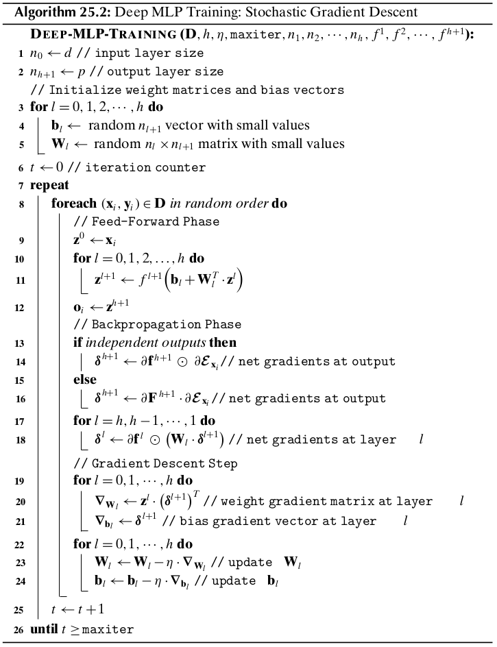
In practice, it is commonto update the gradients by considering a fixed sized subset of the training points called a minibatch instead of using single points. That is, the training data is divided into minibatches using an additional parameter called batch size, and a gradient descent step is performed after computing the bias and weight gradient from each minibatch. This helps better estimate the gradients, and also allows vectorized matrix operations over the minibatch of points, which can lead to faster convergence and substantial speedups in the learning.

One caveat while training very deep MLPs is the problem of vanishing and exploding gradients. In the vanishing gradient problem, the norm of the net gradient can decay exponentially with the distance from the output layer, that is, as we backpropagate the gradients from the output layer to the input layer. In this case the network will learn extremely slowly, if at all, since the gradient descent method will make minuscule changes to the weights and biases. On the other hand, in the exploding gradient problem, the norm of the net gradient can grow exponentially with the distance from the output layer. In this case, the weights and biases will become exponentially large, resulting in a failure to learn. The gradient explosion problem can be mitigated to some extent by gradient thresholding, that is, by resetting the value if itexceeds an upper bound. The vanishing gradients problem is more difficult to address. Typically sigmoid activations are more susceptible to this problem, and one solution is to use a lternative activation functions such as ReLU. In general, recurrent neural networks, which are deep neural networks with feedback connections, are more prone to vanishing and exploding gradients.